 Ali Kamaly
Tektronix TekScope Alternatives in 2026 (Free & Cross-Vendor Analysis)
TekScope brings scope analysis to the desktop, for a licence, on Tektronix files. Here is what it does, where it stops, and the free alternatives for offline waveform analysis.
TekScope brings the Tektronix oscilloscope analysis environment onto a PC, so waveforms captured earlier can be measured, analysed, and reported on without occupying the instrument. TekScope Anywhere is the desktop product.
The motivation is sound: the scope is a shared resource with a small screen, and analysis does not need to happen at the bench. The limits are that it is licensed, it is Tektronix-oriented, and the analysis is not scriptable in the way a real analysis environment is.
What TekScope is good at
- •Familiarity. It is the instrument's own measurement environment, so an engineer who knows the scope knows the software. Nothing to learn.
- •Matching measurements exactly. A measurement taken in TekScope agrees with the one taken on the instrument, because it is the same code. When a number is disputed, this matters.
- •Freeing the bench. The scope keeps capturing while analysis happens elsewhere.
- •Advanced analysis packages for jitter, power, and serial standards, matching what is available on the instrument.
That third point is the real operational value in a busy lab, and it is often enough on its own to justify the licence.
Where it stops
- •It is licensed, and the advanced packages are licensed separately, exactly as on the instrument.
- •It is Tektronix-shaped. Native file formats and workflows assume Tektronix hardware, which is a problem on the mixed benches most labs actually run.
- •It is not scriptable in a general sense. You cannot easily express "process these 500 captures, extract the rise time on each, and flag anything above 4 ns" as code you can review and rerun.
- •The analysis is not version-controlled. A measurement configuration is settings in an application, not a file in a repository.
That third point is where teams outgrow it. Analysis of one waveform is a GUI job. Analysis of 500 is a programming job.
The alternatives
1. Python with numpy, scipy, and matplotlib
Free, and considerably deeper than any scope's built-in analysis.
import numpy as np
from scipy import signal

data = np.loadtxt("capture.csv", delimiter=",", skiprows=1)
t, v = data[:, 0], data[:, 1]

# Rise time, 10 to 90 percent
low, high = np.min(v), np.max(v)
v10, v90 = low + 0.1 * (high - low), low + 0.9 * (high - low)
i10 = np.argmax(v >= v10)
i90 = np.argmax(v >= v90)
print(f"rise time {(t[i90] - t[i10]) * 1e9:.2f} ns")

# Overshoot
settled = np.mean(v[int(len(v) * 0.8):])
print(f"overshoot {100 * (high - settled) / settled:.2f}%")

# Spectrum, which no scope does as well
freqs, psd = signal.welch(v, fs=1 / (t[1] - t[0]), nperseg=4096)
peak = freqs[np.argmax(psd)]
print(f"dominant component at {peak / 1e6:.3f} MHz")
Good for: anything repeated, anything batched, anything needing real signal processing. scipy.signal covers filter design, spectral estimation, and correlation more thoroughly than scope software does.
Gives up: the point-and-click exploration. You are writing code rather than dragging cursors.
Verdict: the default for anything past a handful of waveforms. Batch processing is where it wins outright:
from pathlib import Path

results = []
for path in sorted(Path("captures").glob("*.csv")):
    t, v = np.loadtxt(path, delimiter=",", skiprows=1, unpack=True)
    results.append({"file": path.name, "rise_ns": rise_time(t, v) * 1e9})

failures = [r for r in results if r["rise_ns"] > 4.0]
print(f"{len(failures)} of {len(results)} exceeded 4 ns")
That loop is the thing TekScope cannot do, and it is what a characterisation campaign actually needs.
2. Reading native Tektronix files directly
You do not have to export to CSV. Open-source parsers read .wfm and .isf files, preserving full resolution and the scaling metadata.
Good for: keeping the instrument's native capture path while analysing in Python, avoiding both the CSV size penalty and any precision loss.
Gives up: nothing significant, other than needing to confirm the parser handles your scope's specific format revision.
Verdict: worth setting up if you capture a lot. CSV export of a 10 million point record is slow and enormous.
3. PicoScope software
Free with Pico hardware, and genuinely good analysis for the price, which is zero.
Good for: teams considering new capture hardware, where good bundled software affects the purchase decision.
Gives up: it needs Pico hardware. It does not help with existing Tektronix captures.
Verdict: relevant at purchase time, not at migration time.
4. Sigrok and PulseView
Free and open source, strongest on logic analysis and protocol decoding, with support for a wide range of hardware.
Good for: digital protocol decode where TekScope's serial packages are licensed extras. The decoder library is extensive and community-maintained.
Gives up: analog measurement depth. It is a logic-first tool.
Verdict: a good free substitute specifically for protocol decode, which is often the licensed package people are trying to avoid buying.
5. MATLAB
Reads scope files, and its signal processing library is deeper than anything else here.
Good for: teams that already own MATLAB and do serious analysis. Jitter, eye diagrams, and modulation analysis are well covered.
Gives up: it is another commercial licence. See MATLAB vs LabVIEW.
Verdict: obvious if the licence already exists, hard to justify buying purely to replace TekScope.
Comparison table
| TekScope | Python | Native parsers | PicoScope | Sigrok | MATLAB | |
|---|---|---|---|---|---|---|
| Cost | Licensed | Free | Free | Free with hardware | Free | Commercial |
| Reads Tektronix files | Native | Via export | Native | No | Limited | Yes |
| Cross-vendor | No | Yes | No | Pico only | Yes | Yes |
| Batch processing | Weak | Excellent | Excellent | Weak | Scriptable | Excellent |
| Signal processing depth | Good | Excellent | N/A | Moderate | Logic focus | Excellent |
| Protocol decode | Licensed packages | Via libraries | N/A | Included | Excellent | Toolboxes |
| Interactive exploration | Excellent | Notebooks | N/A | Good | Good | Good |
| Version-controllable | No | Yes | Yes | No | Partly | Yes |
The workflow most labs land on
Not a single tool, and this combination is worth stating because it is what works:
- •Capture on the instrument, scripted, with filenames encoding the conditions. See automating a Tektronix oscilloscope.
- •Explore interactively in TekScope or on the instrument when something looks odd and you do not yet know what you are looking for.
- •Analyse in bulk in Python, with the analysis in version control alongside the test.
- •Report from the analysis output, not by pasting screenshots. See automated test report generation.
The division is between exploration, which is a GUI activity, and measurement, which should be code. TekScope is good at the first and the wrong shape for the second, and most frustration with it comes from using it for the second.
The filename point, again
Worth repeating because it is the cheapest improvement available. A capture named tek0042.wfm is worthless in three months. One named ripple_vin3v3_iout500ma_85c_unit07.wfm is evidence.
Generate the name from the loop that set the conditions, and no capture can ever be mislabelled. That single habit makes batch analysis possible, because the conditions are parseable from the filename:
import re
pattern = re.compile(r"vin(?P<vin>[\\d p]+)_iout(?P<iout>\\d+)ma_(?P<temp>\\d+)c")
Without it, batch analysis requires a separate log correlating filenames to conditions, and that log is always incomplete.
Reading a Tektronix .wfm file in Python
The step that removes the CSV bottleneck entirely. Native files keep full resolution and carry the scaling metadata with them.
import numpy as np

def read_isf(path: str):
    """Parse a Tektronix .isf file into time and voltage arrays."""
    with open(path, "rb") as f:
        raw = f.read()

    header_end = raw.index(b":CURVE #") + len(b":CURVE #")
    header = raw[:header_end].decode("ascii", "ignore")

    def field(name: str, cast=float):
        marker = f"{name} "
        start = header.index(marker) + len(marker)
        end = min(x for x in (header.find(";", start), header.find(":", start)) if x > 0)
        return cast(header[start:end].strip())

    ymult = field("YMULT"); yoff = field("YOFF"); yzero = field("YZERO")
    xincr = field("XINCR"); xzero = field("XZERO")

    digits = int(chr(raw[header_end]))
    length = int(raw[header_end + 1:header_end + 1 + digits])
    data_start = header_end + 1 + digits

    samples = np.frombuffer(raw[data_start:data_start + length], dtype=">i2")
    volts = (samples.astype(float) - yoff) * ymult + yzero
    times = xzero + np.arange(len(volts)) * xincr
    return times, volts
Two orders of magnitude smaller than the CSV of the same record, and no precision lost in decimal formatting. For a campaign capturing hundreds of waveforms, this is the difference between a manageable dataset and a full disk.
Confirm the byte order and word size against your specific scope's programming guide, since older families differ.
Deciding what to keep
Waveform archives grow faster than anyone plans for. A policy set early is worth more than storage bought later.
- •Keep every raw capture that produced a reported number. These are evidence and they must survive as long as the report does.
- •Keep the extracted measurements permanently. They are tiny, and they are what you will actually query in a year.
- •Keep exploratory captures for one project cycle, then delete. Nobody has ever gone back to a debugging capture from two years ago.
- •Never keep a capture without its conditions. An unlabelled waveform is not data, and storing it is worse than deleting it because it implies a record exists.
The practical shape is a directory per run, containing the raw captures, a measurements.csv of extracted values, and the report. Archive the whole directory, prune raw captures on a schedule, and keep the measurements forever.
What a scope-analysis stack actually needs to do
TekScope-class tools all try to cover the same five jobs. Sorting your own need against this list is faster than comparing feature matrices, because most teams need three of the five and buy for all five.
| Job | What it means | Who does it well |
|---|---|---|
| Live view of the front panel | Mirror the scope screen on a PC | Vendor tools, natively |
| Screenshot capture | A PNG for a report or an email | Any tool, and HARDCopy over SCPI |
| Waveform export | Raw samples out as CSV or binary | SCPI CURVe?, or the vendor tool |
| Offline analysis | Maths on captured data after the fact | Python with NumPy, comfortably |
| Automated capture in a sequence | Trigger, wait, capture, measure, log, repeat | Code, or a sequencer |
The split is clean: the first two are what vendor tools are genuinely good at, the last two are what they are structurally bad at, and the middle one is a wash. If your daily work is rows four and five, no vendor scope utility will fit, and that is the case for anyone doing repeated characterisation rather than debug.
Capturing a waveform properly over SCPI
The part people get wrong is the preamble. CURVe? returns integers, not volts, and turning them back into volts needs the scaling factors the scope reports separately.
import numpy as np

scope.write("DATa:SOUrce CH1")
scope.write("DATa:ENCdg RIBinary")     # signed big-endian binary
scope.write("DATa:WIDth 2")            # 16-bit
scope.write("DATa:STARt 1")
scope.write("DATa:STOP 100000")

ymult = float(scope.query("WFMOutpre:YMUlt?"))
yoff  = float(scope.query("WFMOutpre:YOFf?"))
yzero = float(scope.query("WFMOutpre:YZEro?"))
xincr = float(scope.query("WFMOutpre:XINcr?"))

raw = scope.query_binary_values("CURVe?", datatype="h", is_big_endian=True,
                                container=np.array)

volts = (raw - yoff) * ymult + yzero
time_s = np.arange(len(volts)) * xincr
Two details that cause most of the confusion. DATa:WIDth 2 gives 16-bit samples and matches datatype="h"; if you set width 1 you must use "b" or the array is garbage. And the three Y factors are not interchangeable: YOFf is in digitiser levels and YZEro is in volts, which is why the formula subtracts one before scaling and adds the other after.
Once this works, everything downstream is NumPy. See automate a Tektronix oscilloscope with Python for the full acquisition sequence and SCPI command cheat sheet for the equivalents on other vendors.
Common mistakes
- •Capturing the screenshot instead of the data. A PNG cannot be re-measured. Capture the waveform, and generate the picture from it if you need one.
- •Forgetting the preamble. Raw
CURVe?output in a spreadsheet looks plausible and is wrong by a scale factor. - •Mismatching `DATa:WIDth` and the datatype. Silent corruption, not an error.
- •Leaving the record length at the front-panel setting. Set
HORizontal:RECOrdlengthexplicitly in the script so the capture is reproducible. - •Not stopping acquisition before reading. Reading while the scope is running can straddle two acquisitions.
ACQuire:STATE STOPfirst. - •Relying on a vendor tool for the repeatable part. Debug in the GUI, automate in code. Mixing the two is where the manual step creeps back in.
Related reading
- •Automate a Tektronix oscilloscope with Python
- •Tektronix OpenChoice alternatives
- •Keysight vs Tektronix oscilloscopes
- •How to automate test reports
- •PyVISA tutorial
- •SCPI command cheat sheet, the commands per instrument class
- •Instrument control with VISA and SCPI, the transport layer
- •Tektronix vs Rigol oscilloscopes, if hardware is also in scope
- •Python instrument control libraries compared, what to build on
- •Free instrument control software, the zero-cost stack
- •GPIB vs USB vs LAN, why transfer speed varies
- •Test sequencer comparison, automating the capture in a sequence
- •Automate a Rigol oscilloscope with Python, the same job on cheaper hardware
- •NI TestStand alternatives, the sequencer around the capture
Where TestFlow fits
Offline analysis is downstream work. The larger cost is usually upstream, in getting the captures taken consistently in the first place.
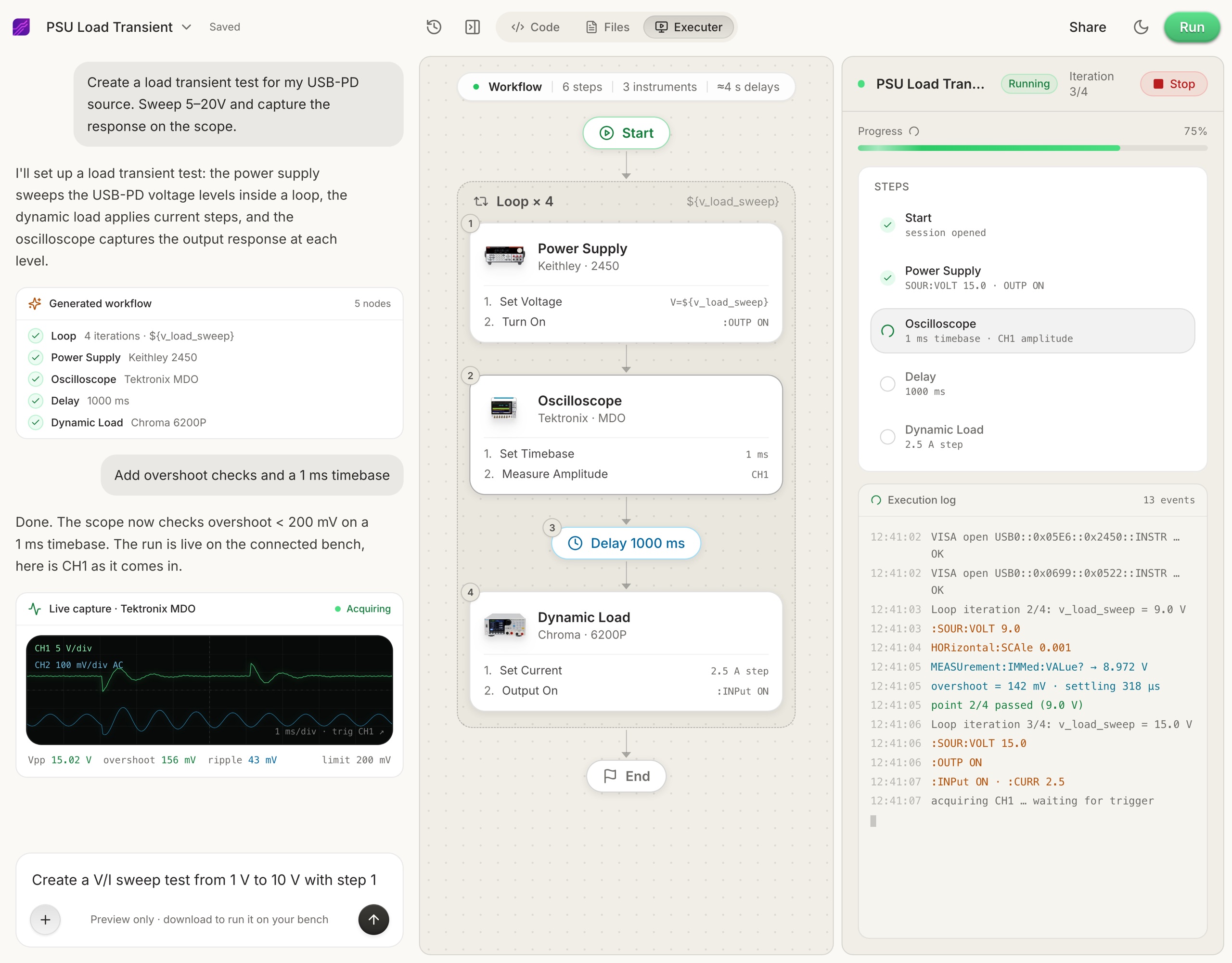
- 1
Connect your instruments. Pick the manufacturer and model, paste the VISA address (USB, LAN, GPIB, or serial), and the agent knows what is on your bench. No bench yet? Use a placeholder address, build the full automation, and swap in the real address when you are in the lab.
- 2
Tell the agent what to test, in plain English. For example, "run a VI sweep from 1 to 10 V in 1 V steps at 0.5 A load current," or "suggest the tests for a power-management device."
- 3
The agent builds the complete workflow in seconds. Instrument-aware automation appears on the canvas, with the generated scripts visible in a code panel you can inspect and edit.
- 4
Run it in your lab. Click Run and the status panel streams results step by step, with measured values inline (VOUT = 3.301 V, asserted 3.2 to 3.4 V, PASS). One click exports a structured PDF report, or the raw results as CSV.
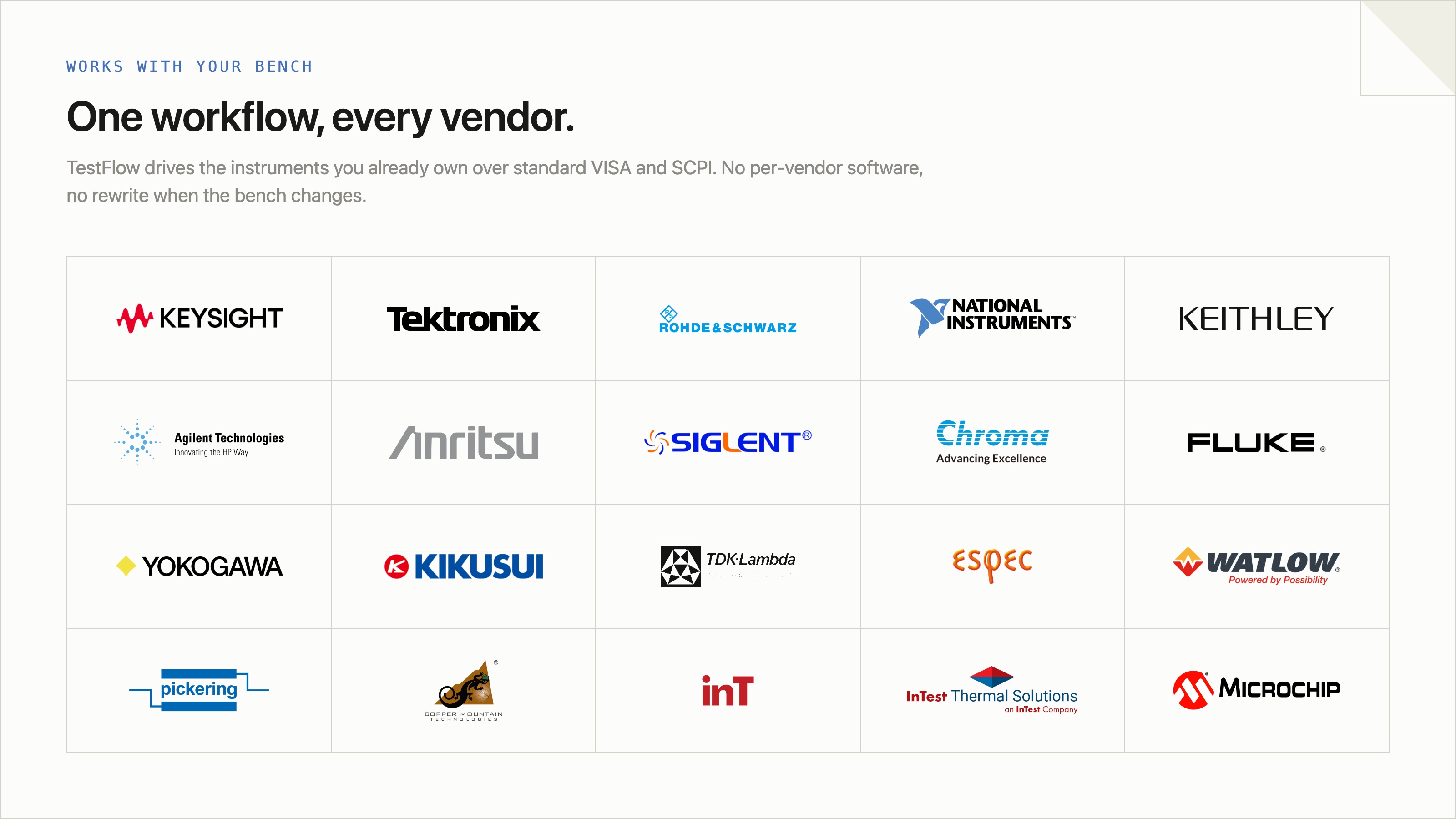
- Vendor-neutral by design. One workflow drives Keysight, Tektronix, Rohde & Schwarz, NI, Rigol, Keithley, Anritsu, and more over standard VISA and SCPI.
- Browser-based and shareable. Workflows live in your workspace, so a sequence built in one lab runs the same way in another.
- Free version to start. Sign in at app.testflowinc.com and build your first workflow today; plans and quotes are on the pricing page.
The step-by-step walkthrough, VISA address formats, and Test Planner prompts are all in the TestFlow product guide.
Frequently asked questions
What is Tektronix TekScope?
Analysis software that brings the oscilloscope's measurement and analysis environment to a PC, so waveforms captured earlier can be examined, measured, and reported on away from the instrument. TekScope Anywhere is the desktop offering.
Is TekScope free?
There is limited free functionality, and the full analysis capability is licensed. Advanced analysis packages such as jitter and power analysis are separately licensed, as they are on the instrument itself.
Can I analyse Tektronix waveform files without TekScope?
Yes. Tektronix .wfm and .isf files can be read with open-source Python parsers, and CSV export from the scope works with any tool. Your captured data is not locked to the software.
What is the best free alternative to TekScope?
Python with numpy, scipy, and matplotlib. It reads exported waveforms, does deeper signal processing than most scope software, and the analysis is scriptable and version-controlled.
Does TekScope work with other vendors' oscilloscopes?
It is built for Tektronix instruments and file formats. For a mixed-vendor bench you need a vendor-neutral analysis path, which in practice means exporting to CSV or a common format and analysing elsewhere.
Why analyse waveforms on a PC rather than on the scope?
The scope is a shared instrument and its screen is small. Moving analysis to a desktop frees the bench, allows batch processing of many captures, and lets the analysis be scripted and repeated identically.
Ready to automate your lab?
Connect your instruments, describe a test in plain English, and TestFlow builds and runs it in minutes.
Tags
Put it on your bench this week
A new way for testing, from specs to automated sequences, capture clean data, and accelerate your validation cycle.