 Ali Kamaly
How to Automate a VI Curve Sweep in 2026 (Power Supply, DMM & Load)
A working guide to automating VI characterisation: instrument roles, why 4-wire matters, how to find the real settling time, safe compliance handling, and a complete script you can adapt.
A VI curve sweep steps a source across a range and records the resulting current or voltage, producing a device's current-voltage characteristic. It is the most common multi-instrument measurement in electronics validation and the first thing most engineers automate.
It is also where three specific mistakes get made every time: measuring at the wrong point, guessing the settling time, and silently recording points taken in compliance. This guide covers the instrument roles, those three problems, and a complete working script.
The instrument roles
| Role | Instrument | Why |
|---|---|---|
| Force | Programmable DC supply | Sets the voltage or current at each step |
| Measure voltage | 6.5-digit DMM, 4-wire | Accurate voltage at the device, not at the supply |
| Measure current | DMM or supply readback | Depends on the accuracy you need |
| Sink | Electronic load | Only when characterising a source such as a converter or cell |
If you own a source measure unit, it does all of this in one box with 4-wire built in, and you should use it. This guide targets the far more common bench that has a supply, a DMM, and possibly a load.
Problem 1: measuring at the wrong point
A supply reports the voltage at its own terminals. Between there and your device sit two lead resistances, and at any meaningful current they produce a real error.
At 500 mA through 100 milliohms of lead and connector resistance, that is 50 mV. On a 3.3 V rail it is a 1.5 percent error, and it changes with current, which means it distorts the shape of the curve rather than just offsetting it.
The fix is 4-wire measurement. Force through one pair, sense through another, connected at the device.
dmm.write("CONF:FRES 100,0.001")     # 4-wire resistance
dmm.write("CONF:VOLT:DC 10,0.00001") # 4-wire voltage uses the sense pair
The sense leads carry almost no current, so they drop almost no voltage, so the DMM reads what the device actually sees.
When you can skip it: measuring high voltages at low current, where lead drop is negligible relative to the value. Everything else, use 4-wire.
Problem 2: guessing the settling time
The single largest source of wasted run time and the second largest source of wrong data.
Too short and you record the previous point's value while the supply is still moving. Too long and a 200-point sweep takes ten minutes instead of one.
Measure it once, properly:
import time

psu.write("VOLT 1.0"); psu.write("OUTP ON")
time.sleep(1)                        # settled at the start point

psu.write("VOLT 3.3")                # the step under test
t0 = time.perf_counter()
samples = []
while time.perf_counter() - t0 < 1.0:
    samples.append((time.perf_counter() - t0, float(dmm.query("READ?"))))

final = samples[-1][1]
for t, v in samples:
    if abs(v - final) < 0.0005:      # within your resolution
        print(f"settled at {t*1000:.0f} ms")
        break
Run that once for your worst-case step and use the answer, with margin. Typical benches find 20 to 60 ms where they had been using 200.
Note that settling depends on the load. Measure it with the device connected, not into an open circuit.
Problem 3: compliance recorded silently
When the supply hits its current limit it stops being a voltage source and becomes a current source. The voltage at the device is then whatever the device does, not what you asked for.
A sweep that walks into compliance records a flat region that looks like a real device characteristic and is not.
def in_compliance(psu) -> bool:
    return bool(int(psu.query("STAT:QUES:COND?")) & 0x02)
Check after every point, record the flag in the data, and decide deliberately whether to stop the sweep or continue with the points marked. Never drop the flag.
Bit definitions vary by model, so confirm against the programming guide for your instrument.
The complete script
import csv
import time
import pyvisa

PSU_ADDR = "TCPIP0::192.168.1.42::inst0::INSTR"
DMM_ADDR = "USB0::0x2A8D::0x1301::MY57200001::INSTR"

V_START, V_STOP, V_STEP = 0.0, 5.0, 0.05
I_LIMIT = 0.5
SETTLE_S = 0.05                      # measured, not guessed

rm = pyvisa.ResourceManager()
psu = rm.open_resource(PSU_ADDR); psu.timeout = 10000
dmm = rm.open_resource(DMM_ADDR); dmm.timeout = 10000


def check(inst, label):
    while True:
        response = inst.query("SYST:ERR?").strip()
        if response.startswith("0,") or response.startswith("+0,"):
            break
        raise RuntimeError(f"{label}: {response}")


def in_compliance(inst) -> bool:
    return bool(int(inst.query("STAT:QUES:COND?")) & 0x02)


rows = []
try:
    print(psu.query("*IDN?").strip())
    print(dmm.query("*IDN?").strip())

    psu.write("*RST"); psu.write("*CLS")
    dmm.write("*RST"); dmm.write("*CLS")

    # DMM: 4-wire DC volts, 1 PLC integration for mains rejection
    dmm.write("CONF:VOLT:DC 10,0.00001")
    dmm.write("VOLT:DC:NPLC 1")
    dmm.write("TRIG:SOUR IMM")
    check(dmm, "dmm")

    psu.write(f"CURR {I_LIMIT}")
    psu.write(f"VOLT {V_START}")
    psu.write("OUTP ON")
    check(psu, "psu")
    time.sleep(0.5)                  # initial settle

    steps = int(round((V_STOP - V_START) / V_STEP)) + 1
    for n in range(steps):
        v_set = V_START + n * V_STEP
        psu.write(f"VOLT {v_set:.4f}")
        time.sleep(SETTLE_S)

        v_meas = float(dmm.query("READ?"))
        i_meas = float(psu.query("MEAS:CURR?"))
        clamped = in_compliance(psu)

        rows.append({
            "v_set": round(v_set, 4),
            "v_meas": v_meas,
            "i_meas": i_meas,
            "p_w": round(v_meas * i_meas, 8),
            "compliance": clamped,
        })

        flag = "  <-- COMPLIANCE" if clamped else ""
        print(f"{v_set:5.2f} V set  {v_meas:9.6f} V  {i_meas*1000:8.3f} mA{flag}")

    check(psu, "psu"); check(dmm, "dmm")

finally:
    psu.write("OUTP OFF")
    psu.close(); dmm.close(); rm.close()

with open("vi_curve.csv", "w", newline="") as f:
    writer = csv.DictWriter(f, fieldnames=list(rows[0].keys()))
    writer.writeheader(); writer.writerows(rows)

bad = [r for r in rows if r["compliance"]]
print(f"\n{len(rows)} points, {len(bad)} in compliance")
if bad:
    print(f"first compliance point at {bad[0]['v_set']} V, curve is invalid beyond it")
What makes this production-grade rather than a demo
Four things, and they are the difference between a script you run once and one you leave running overnight.
- •`try/finally` around everything. The output is disabled even if a step raises. Without this a crash leaves the device powered at whatever the last setpoint was.
- •Integer step counting.
for n in range(steps)rather than accumulating a float. Floating-point accumulation drops or duplicates the final point roughly half the time. - •Error queue checked before and after the sweep, so a rejected command surfaces rather than producing quietly wrong data.
- •Compliance recorded per point, not discarded.
Sweeping current instead of voltage
For diodes and LEDs you usually want to source current and measure voltage, which is the same structure with the roles swapped:
psu.write(f"VOLT {V_MAX}")           # voltage becomes the compliance limit
psu.write(f"CURR {i_set:.6f}")       # current is now the swept variable
Set the voltage limit to something the device survives. For an LED, forward voltage plus a small margin.
Bidirectional sweeps for hysteresis
Devices with hysteresis, and any measurement where self-heating matters, need the sweep run in both directions:
forward = [V_START + n * V_STEP for n in range(steps)]
for direction, points in (("up", forward), ("down", list(reversed(forward)))):
    for v_set in points:
        ...
        rows.append({..., "direction": direction})
If the up and down curves differ by more than your measurement uncertainty, you have either genuine hysteresis or a settling time that is still too short. Checking which is the point of running it.
Adding an electronic load for source characterisation
Everything above sweeps a source into a passive device. Characterising a source, a converter, a regulator, or a cell, means sweeping the load instead.
load.write("FUNC CURR")               # constant current mode
load.write("CURR 0")
load.write("INP ON")

rows = []
for i_set in [0.0, 0.1, 0.25, 0.5, 0.75, 1.0, 1.5, 2.0]:
    load.write(f"CURR {i_set:.4f}")
    time.sleep(SETTLE_S)

    v_out = float(dmm.query("READ?"))          # 4-wire at the DUT terminals
    i_actual = float(load.query("MEAS:CURR?"))
    rows.append({"i_set": i_set, "v_out": v_out, "i_actual": i_actual,
                 "p_w": v_out * i_actual})
    print(f"{i_set:5.2f} A  ->  {v_out:.5f} V   {v_out*i_actual:7.3f} W")

load.write("INP OFF")
Note the load uses INP rather than OUTP. Sending OUTP ON to a load is a common error that produces no effect and no obvious message.
Load regulation falls straight out of this data:
v_noload = rows[0]["v_out"]
v_fullload = rows[-1]["v_out"]
regulation_pct = 100 * (v_noload - v_fullload) / v_noload
print(f"load regulation {regulation_pct:.3f}% from 0 to {rows[-1]['i_set']} A")
Watch the power dissipation. A load sinking 2 A from a 12 V source dissipates 24 W, and benchtop loads have both a power limit and a thermal time constant. Sweeping to full current and holding there while the script does something else is how loads get thermally shut down mid-run. Step down to zero between points if the sweep is slow.
Plotting and finding the knee
import matplotlib.pyplot as plt

v = [r["v_meas"] for r in rows]
i = [r["i_meas"] for r in rows]

fig, ax = plt.subplots(figsize=(7, 4.5))
ax.plot(v, [x * 1000 for x in i], marker=".", linewidth=1)
ax.set_xlabel("Voltage (V)"); ax.set_ylabel("Current (mA)")
ax.grid(alpha=0.3)
fig.savefig("vi_curve.png", dpi=150, bbox_inches="tight")
For a diode, finding the forward knee is a derivative rather than a threshold:
import numpy as np
di_dv = np.gradient(np.array(i), np.array(v))
knee_index = int(np.argmax(di_dv > 0.001))
print(f"knee at {v[knee_index]:.4f} V")
Using the gradient rather than a fixed current threshold makes the measurement independent of the current range, which matters when comparing devices of different sizes.
Turning the sweep into a pass or fail
A curve is data. A verdict is a result. The step between them is where most home-grown sweeps stop, and it is the step that makes the run useful to anyone who was not in the lab that day.
from dataclasses import dataclass

@dataclass
class Limit:
    name: str
    lo: float
    hi: float
    units: str

LIMITS = [
    Limit("vout_nominal", 3.20, 3.40, "V"),
    Limit("load_regulation_pct", -1.0, 1.0, "%"),
    Limit("efficiency_at_full_load", 0.85, 1.00, ""),
]

def evaluate(metrics: dict, limits: list[Limit]) -> tuple[str, list[dict]]:
    rows = []
    for lim in limits:
        value = metrics[lim.name]
        ok = lim.lo <= value <= lim.hi
        rows.append({
            "parameter": lim.name, "measured": value, "units": lim.units,
            "limits": f"{lim.lo} to {lim.hi}", "verdict": "PASS" if ok else "FAIL",
        })
    overall = "PASS" if all(r["verdict"] == "PASS" for r in rows) else "FAIL"
    return overall, rows
Two rules that keep this maintainable. Limits live in data, never inline in the sweep, so a new silicon revision is a new file rather than a code change. And the evaluation records the limits it used alongside the measurement, so a report from six months ago still explains itself. That second point is what an auditor asks for and what a bare CSV cannot answer. See automated test report generation for the document stage.
Sweep resolution and how long the run takes
The parameter that decides run time, and the one most often chosen by habit rather than by need.
| Step size over a 0 to 10 V sweep | Points | At 0.5 s settle | When it is right |
|---|---|---|---|
| 1.0 V | 11 | 6 s | Smoke test, does the rail come up |
| 0.5 V | 21 | 11 s | Routine regression |
| 0.1 V | 101 | 51 s | Characterisation, finding the knee |
| 0.02 V | 501 | 4 min | Resolving a sharp transition |
| 0.01 V | 1001 | 8 min | Rarely justified outside a knee region |
The efficient pattern is two passes rather than one fine sweep: a coarse pass to find where the curve bends, then a fine pass over only that region. A 10 V characterisation that would take eight minutes at uniform fine resolution takes about ninety seconds when the fine points are spent only where the curve is actually doing something.
Settling time dominates the total, not the measurement, which is why the settling discussion earlier in this post matters more than the sample rate of the DMM.
Common mistakes
- •Measuring at the supply rather than the DUT. Covered above. Lead drop at any real current is not negligible.
- •A fixed settle for the whole sweep. The first point after output-on needs longer than the rest. Handle the first point separately.
- •Not recording compliance state. A supply in constant current is not delivering the voltage you asked for, and a curve that ignores this is silently wrong.
- •Uniform fine resolution. Two passes, as above.
- •Leaving the output on between sweeps. Between test cases, output off. It costs a second and prevents a class of accidents.
- •Sweeping up only. If the DUT has hysteresis, an up-only sweep hides it. Sweep both directions when the device has any latching or thermal behaviour.
- •Storing only the summary. Keep the raw points. Regenerating a summary from raw data is trivial; recovering raw data from a summary is impossible.
Related reading
- •Automate a Keysight power supply with Python
- •Automate multimeter measurements with Python
- •PyVISA tutorial
- •SCPI command cheat sheet
- •Programmable DC power supply, choosing the hardware
- •Automated test report generation, turning the curve into a document
- •Instrument control with VISA and SCPI, the protocol layer
- •Read a digital multimeter datasheet, how accurate the points really are
- •Test sequencer comparison, running this as one step of many
- •Optimizing test coverage, choosing which sweeps to run
- •Python instrument control libraries compared, what to build on
- •GPIB vs USB vs LAN, the interface underneath
- •Free instrument control software, the zero-cost stack
- •Hardware testing best practices, the wider discipline
- •NI TestStand alternatives, if the sweep is one step in a longer sequence
Where TestFlow fits
A VI sweep is the simplest multi-instrument test there is, and it still takes most engineers a day to build reliably. That gap is what an agent removes.
- 1
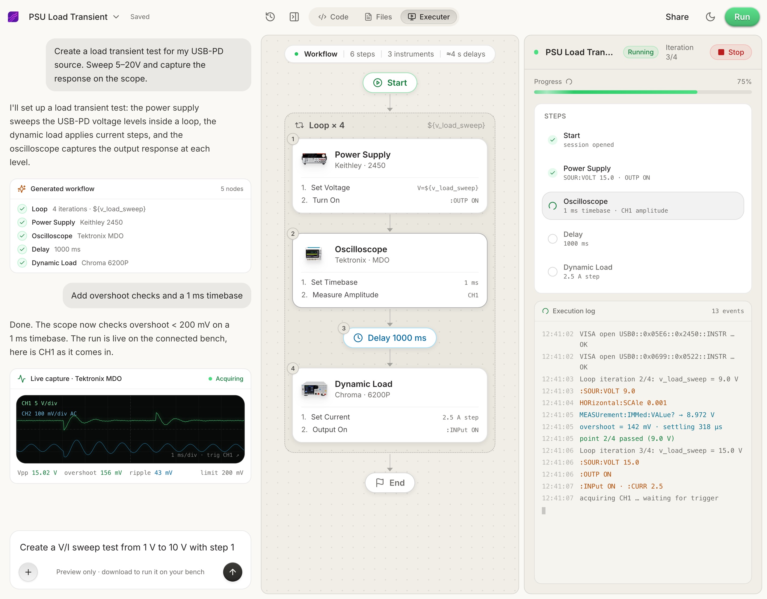
Connect your instruments. Pick the manufacturer and model, paste the VISA address (USB, LAN, GPIB, or serial), and the agent knows what is on your bench. No bench yet? Use a placeholder address, build the full automation, and swap in the real address when you are in the lab.
- 2
Tell the agent what to test, in plain English. For example, "run a VI sweep from 1 to 10 V in 1 V steps at 0.5 A load current," or "suggest the tests for a power-management device."
- 3
The agent builds the complete workflow in seconds. Instrument-aware automation appears on the canvas, with the generated scripts visible in a code panel you can inspect and edit.
- 4
Run it in your lab. Click Run and the status panel streams results step by step, with measured values inline (VOUT = 3.301 V, asserted 3.2 to 3.4 V, PASS). One click exports a structured PDF report, or the raw results as CSV.
- Vendor-neutral by design. One workflow drives Keysight, Tektronix, Rohde & Schwarz, NI, Rigol, Keithley, Anritsu, and more over standard VISA and SCPI.
- Browser-based and shareable. Workflows live in your workspace, so a sequence built in one lab runs the same way in another.
- Free version to start. Sign in at app.testflowinc.com and build your first workflow today; plans and quotes are on the pricing page.

The step-by-step walkthrough, VISA address formats, and Test Planner prompts are all in the TestFlow product guide.
Frequently asked questions
What is a VI curve sweep?
A measurement that steps voltage or current across a range and records the resulting current or voltage, producing the current-voltage characteristic of a device. It is the basic characterisation measurement for diodes, transistors, solar cells, LEDs, and power converters.
Why use a separate DMM instead of the power supply's own readback?
A supply's internal readback is typically 3 to 4 digits and measures at its own terminals, so it includes lead drop. A 6.5-digit DMM measuring 4-wire at the device gives far better accuracy and removes cable resistance from the result.
What is 4-wire measurement and when do I need it?
Four-wire, or Kelvin, measurement uses separate pairs for forcing current and sensing voltage, so the voltage is measured at the device rather than after the leads. Use it whenever measuring low voltages, low resistances, or drawing more than a few tens of milliamps.
How long should I wait between sweep points?
Measure it rather than guessing. Step the source, then poll the meter in a tight loop with timestamps and see when the reading stabilises to within your resolution. Most benches find the real number is well under the 200 ms people default to.
How do I handle compliance during a sweep?
Set the current limit before each step, and after each measurement check whether the source entered constant-current mode with STAT:QUES:COND?. A point taken in compliance is not on the curve you think it is and should be flagged, not silently recorded.
Can I do a VI sweep with just an SMU?
Yes, and it is simpler. A source measure unit sources and measures in one instrument with 4-wire built in. The three-instrument approach in this guide is for benches that have a supply, DMM, and load rather than an SMU.
Ready to automate your lab?
Connect your instruments, describe a test in plain English, and TestFlow builds and runs it in minutes.
Tags
Put it on your bench this week
A new way for testing, from specs to automated sequences, capture clean data, and accelerate your validation cycle.