 Ali Kamaly
Automate a Tektronix Function Generator with Python (AFG31000, 2026)
Driving a Tektronix AFG from Python: the commands that matter, the output impedance mistake that doubles your amplitude, sweeps, bursts, and uploading arbitrary waveforms.
A Tektronix function generator is controlled from Python with PyVISA over USB or LAN, using the SOURce and OUTPut SCPI subsystems. The commands are straightforward. The one thing that catches almost everyone is the output impedance setting, which silently doubles your amplitude when it is wrong.
This guide covers connection, basic waveforms, the impedance trap, sweeps, bursts, and uploading arbitrary waveforms.
Connect
import pyvisa

rm = pyvisa.ResourceManager()
afg = rm.open_resource("TCPIP0::192.168.1.55::inst0::INSTR")
afg.timeout = 10000

print(afg.query("*IDN?").strip())
afg.write("*RST")
afg.write("*CLS")
Expect something like:
TEKTRONIX,AFG31052,SERIAL,SCPI:99.0 FV:1.4.2Tektronix USB devices use vendor ID 0x0699. See the PyVISA tutorial for backend setup.
The impedance trap, first
Deal with this before anything else, because every amplitude you set depends on it.
A function generator has a 50 ohm source impedance. It computes the output voltage assuming a matched 50 ohm load, which forms a divider halving the open-circuit voltage. Connect a high-impedance load instead, such as a scope input at 1 megohm, and there is no divider, so you get exactly twice what you asked for.
afg.write("OUTPut1:IMPedance INFinity")   # for scope inputs, high-Z circuits
# or
afg.write("OUTPut1:IMPedance 50")         # for a real 50 ohm termination
Set it explicitly, every time, as the first thing after *RST. Do not rely on the default and do not rely on what the last person left it at.
The symptom of getting this wrong is a measurement that is consistently off by a factor of two, which people usually attribute to a probe setting or a scale error and spend an hour chasing.
Basic waveform output
afg.write("OUTPut1:IMPedance INFinity")
afg.write("SOURce1:FUNCtion SIN")
afg.write("SOURce1:FREQuency 1E3")
afg.write("SOURce1:VOLTage 2.0")          # 2 Vpp
afg.write("SOURce1:VOLTage:OFFSet 0")
afg.write("OUTPut1:STATe ON")
The commands that matter:
| Command | Purpose | ||
|---|---|---|---|
SOURce1:FUNCtion <shape> | SIN, SQU, RAMP, PULS, NOIS, DC, USER | ||
SOURce1:FREQuency <hz> | Frequency | ||
SOURce1:VOLTage <vpp> | Amplitude, peak to peak by default | ||
SOURce1:VOLTage:OFFSet <v> | DC offset | ||
| `SOURce1:VOLTage:UNIT VPP\ | VRMS\ | DBM` | Amplitude units |
SOURce1:PHASe:ADJust <deg> | Phase | ||
SOURce1:FUNCtion:PULSe:DCYCle <pct> | Pulse duty cycle | ||
| `OUTPut1:STATe ON\ | OFF` | Enable output | |
| `OUTPut1:IMPedance 50\ | INFinity` | Load assumption |
Channel 2 on dual-output models is the same with SOURce2 and OUTPut2.
Verify what you set
Generators clamp silently when a request exceeds a limit, exactly like power supplies.
def set_and_verify(inst, command: str, query: str, wanted: float, tol: float = 1e-6):
    inst.write(f"{command} {wanted}")
    actual = float(inst.query(query))
    if abs(actual - wanted) > tol:
        raise RuntimeError(f"{command}: asked {wanted}, instrument set {actual}")
    return actual

set_and_verify(afg, "SOURce1:FREQuency", "SOURce1:FREQuency?", 1e3)
set_and_verify(afg, "SOURce1:VOLTage", "SOURce1:VOLTage?", 2.0, tol=1e-4)
Amplitude limits depend on the impedance setting and the offset, so a value that is legal at one offset can be clamped at another. Verifying catches this.
Frequency sweeps
Two approaches, and the choice matters.
Instrument-driven sweep, where the generator handles the timing:
afg.write("SOURce1:FREQuency:STARt 100")
afg.write("SOURce1:FREQuency:STOP 100E3")
afg.write("SOURce1:SWEep:TIME 1")
afg.write("SOURce1:SWEep:SPACing LOGarithmic")
afg.write("SOURce1:FREQuency:MODE SWEep")
afg.write("OUTPut1:STATe ON")
Smooth and fast, and you cannot take a settled measurement at each point because the frequency is always moving.
Script-driven stepping, which is what you want for a frequency response measurement:
import time
import numpy as np

frequencies = np.logspace(2, 5, 61)          # 100 Hz to 100 kHz, 61 points
results = []

afg.write("SOURce1:FREQuency:MODE CW")
afg.write("OUTPut1:STATe ON")

for frequency in frequencies:
    afg.write(f"SOURce1:FREQuency {frequency:.6E}")
    time.sleep(0.05)                          # settle, measured not guessed
    amplitude = float(scope.query("MEASUREMENT:IMMED:VALUE?"))
    results.append((frequency, amplitude))
    print(f"{frequency:10.1f} Hz  {amplitude:.4f} V")

afg.write("OUTPut1:STATe OFF")
Use logspace rather than linspace for anything with frequency-dependent behaviour. A linear sweep from 100 Hz to 100 kHz puts almost every point above 50 kHz and tells you nothing about the low end.
Burst mode
For transient response and for stimulating a device a defined number of cycles.
afg.write("SOURce1:FUNCtion SIN")
afg.write("SOURce1:FREQuency 10E3")
afg.write("SOURce1:VOLTage 1.0")
afg.write("SOURce1:BURSt:MODE TRIGgered")
afg.write("SOURce1:BURSt:NCYCles 5")
afg.write("SOURce1:BURSt:STATe ON")
afg.write("TRIGger:SEQuence:SOURce EXTernal")   # or MANual for software trigger
afg.write("OUTPut1:STATe ON")

afg.write("*TRG")                               # fire one burst
For repeatable capture, trigger the scope from the generator's sync output rather than trying to trigger on the signal itself. The sync output is a clean logic-level edge coincident with the burst start, which removes an entire class of unstable-trigger problems.
Arbitrary waveforms
Upload your own samples for tests that need a specific stimulus, a recorded transient, or a modulated signal.
import numpy as np

# Build the waveform, here a sine with a glitch
n = 8192
t = np.linspace(0, 1, n, endpoint=False)
wave = np.sin(2 * np.pi * t)
wave[4000:4020] += 0.4                          # the injected glitch

# Normalise to the instrument's signed 14-bit range
wave = wave / np.max(np.abs(wave))
samples = (wave * 8191).astype(np.int16)

afg.write("SOURce1:FUNCtion:SHAPe EMEMory")
afg.write_binary_values("DATA:DATA EMEMory,", samples,
                        datatype="h", is_big_endian=True)

afg.write("SOURce1:FREQuency 1E3")
afg.write("SOURce1:VOLTage 2.0")
afg.write("OUTPut1:STATe ON")
Three details that matter:
- •Normalise before converting. The instrument scales the integer range to the amplitude you set, so the samples define the shape and
SOURce1:VOLTagedefines the size. - •Match the datatype and endianness to what the instrument expects.
"h"is a signed 16-bit integer, and Tektronix generally expects big-endian here. - •The frequency now means the repetition rate of the whole waveform, not the frequency of anything inside it. A 8192-point waveform at 1 kHz plays 8192 samples in 1 ms.
Check the memory depth for your specific model before generating a large waveform, since the AFG1000 and AFG31000 series differ substantially.
A complete frequency response measurement
Putting it together, the generator and a scope measuring a filter:
import time
import csv
import numpy as np

afg.write("*RST"); afg.write("OUTPut1:IMPedance INFinity")
afg.write("SOURce1:FUNCtion SIN")
afg.write("SOURce1:VOLTage 1.0")
afg.write("SOURce1:FREQuency:MODE CW")
afg.write("OUTPut1:STATe ON")

rows = []
try:
    for frequency in np.logspace(2, 5, 61):
        afg.write(f"SOURce1:FREQuency {frequency:.6E}")
        scope.write(f"HORIZONTAL:SCALE {1/(frequency*10):.6E}")
        time.sleep(0.1)
        vout = float(scope.query("MEASUREMENT:IMMED:VALUE?"))
        gain_db = 20 * np.log10(vout / 1.0)
        rows.append({"hz": frequency, "vout": vout, "gain_db": gain_db})
        print(f"{frequency:9.1f} Hz  {gain_db:7.2f} dB")
finally:
    afg.write("OUTPut1:STATe OFF")

with open("response.csv", "w", newline="") as f:
    w = csv.DictWriter(f, fieldnames=["hz", "vout", "gain_db"])
    w.writeheader(); w.writerows(rows)

cutoff = next((r for r in rows if r["gain_db"] <= -3), None)
if cutoff:
    print(f"-3 dB at {cutoff['hz']:.0f} Hz")
Note the scope timebase being rescaled with the frequency. Leaving it fixed means the measurement is taken on a waveform that is either a flat line or a solid block for most of the sweep, which is the second most common mistake in this measurement after the impedance setting.
Modulation and two-channel work
Dual-output models let you drive a device and provide a reference or a trigger from the same instrument, which removes a whole class of synchronisation problems.
afg.write("SOURce1:FUNCtion SIN")
afg.write("SOURce1:FREQuency 1E4")
afg.write("SOURce2:FUNCtion SQU")
afg.write("SOURce2:FREQuency 1E4")
afg.write("SOURce2:VOLTage 3.3")
afg.write("SOURce2:VOLTage:OFFSet 1.65")   # 0 to 3.3 V logic-level reference

afg.write("SOURce1:PHASe:INITiate")        # align the two channels
afg.write("OUTPut1:STATe ON")
afg.write("OUTPut2:STATe ON")
SOURce1:PHASe:INITiate resets the phase relationship between channels. Without it the two outputs start at an arbitrary relative phase, which makes any timing measurement between them meaningless and, worse, different on every run.
Built-in modulation covers common stimulus needs without uploading an arbitrary waveform:
afg.write("SOURce1:AM:STATe ON")
afg.write("SOURce1:AM:SOURce INTernal")
afg.write("SOURce1:AM:INTernal:FUNCtion SIN")
afg.write("SOURce1:AM:INTernal:FREQuency 100")
afg.write("SOURce1:AM:DEPTh 50")
Frequency and phase modulation follow the same pattern with FM and PM in place of AM.
Checking errors, and a safe wrapper
Generators queue errors silently exactly like every other SCPI instrument.
def check(inst) -> None:
    problems = []
    while True:
        response = inst.query("SYSTem:ERRor?").strip()
        if response.startswith(("0,", "+0,")):
            break
        problems.append(response)
        if len(problems) > 20:
            break
    if problems:
        raise RuntimeError("AFG errors: " + "; ".join(problems))
And wrap any session that enables an output so it cannot be left driving a device:
from contextlib import contextmanager

@contextmanager
def output_enabled(inst, channel: int = 1):
    inst.write(f"OUTPut{channel}:STATe ON")
    try:
        yield inst
    finally:
        inst.write(f"OUTPut{channel}:STATe OFF")

with output_enabled(afg):
    run_frequency_sweep(afg, scope)
A generator left running into a powered-down device can forward-bias protection diodes through the input, which is a real way to damage a board overnight. The context manager makes forgetting impossible rather than unlikely.
Synchronising the generator with the measurement
A frequency response run is only as good as its settling discipline. The generator changes frequency in microseconds; the DUT, the filter, and the measuring instrument do not.
def settle_and_measure(afg, dmm, freq_hz, cycles=50, min_wait=0.05):
    afg.write(f"SOUR1:FREQ {freq_hz:g}")
    afg.query("*OPC?")                      # generator has applied the setting
    wait = max(cycles / freq_hz, min_wait)  # scale the wait with the period
    time.sleep(wait)
    return float(dmm.query("READ?"))
Scaling the wait with the period is the part that is usually missing. A fixed 100 ms sleep is generous at 10 kHz and far too short at 10 Hz, which is why low-frequency points on a hand-written sweep so often look wrong. Waiting a fixed number of cycles fixes the whole sweep with one line.
*OPC? after the frequency write confirms the generator has processed the command rather than merely received it. On a USB connection the difference is negligible; over LAN with a busy instrument it is not.
Output state and safety
Function generators do less damage than power supplies, but the same discipline applies and costs nothing.
try:
    afg.write("OUTP1:STAT ON")
    run_sweep(afg, dmm)
finally:
    afg.write("OUTP1:STAT OFF")
    afg.write("OUTP2:STAT OFF")
    afg.close()
Two model-specific points worth checking before an unattended run. Some AFG models restore the previous output state on power-up, so a mains blip can re-energise an output you thought was off. And *RST sets the amplitude to a default that may be larger than what your DUT tolerates, so set amplitude and offset explicitly after every reset rather than assuming a safe default.
Common mistakes
- •The impedance mismatch. Covered above, and it is the single most common cause of a signal that is exactly double or half what you expected.
- •A fixed settling delay across a wide sweep. Scale it with the period, as above.
- •Setting frequency without setting amplitude after a reset.
*RSTdefaults are not your defaults. - •Assuming the generator's amplitude is what the DUT sees. Cable loss and load impedance both matter. Measure at the DUT for anything above a few MHz.
- •Using `time.sleep()` where the instrument offers a trigger. Burst and sweep modes have hardware triggering that is more repeatable than an OS timer.
- •Not checking `SYST:ERR?` after configuration. A rejected command leaves the instrument on the previous setting and says nothing.
- •Loading an arbitrary waveform without normalising it. The DAC expects a normalised range. Feeding raw volts produces clipping that looks like a DUT fault.
Related reading
- •Automate a Tektronix oscilloscope with Python
- •PyVISA tutorial
- •SCPI command cheat sheet
- •Function generator specifications
- •Best function and signal generator
- •Keysight 33600A programming, the same job on Keysight hardware
- •Instrument control with VISA and SCPI, the protocol layer
- •Automate multimeter measurements with Python, the measurement half
- •GPIB vs USB vs LAN, picking the interface
- •Automate a Keysight power supply with Python, the third instrument in most setups
- •Python instrument control libraries compared, what to build on
- •Automated test report generation, turning a sweep into a document
- •Free instrument control software, the zero-cost stack
- •Test sequencer comparison, running the sweep inside a sequence
- •NI TestStand alternatives, the commercial sequencer for production runs
Where TestFlow fits
A signal generator is only useful paired with a measurement. The sequencing between them is the part that takes an afternoon to write and thirty seconds to describe.
- 1
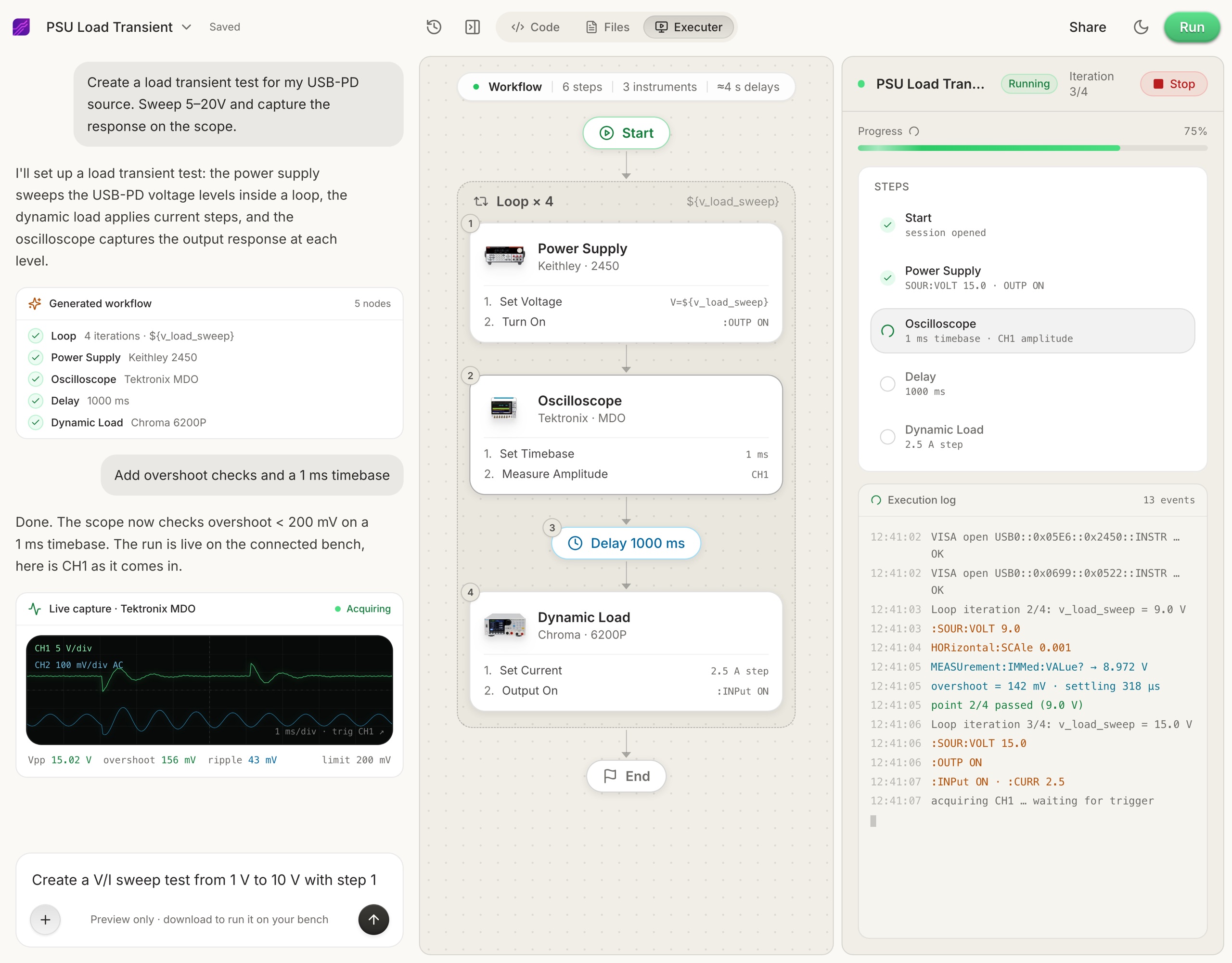
Connect your instruments. Pick the manufacturer and model, paste the VISA address (USB, LAN, GPIB, or serial), and the agent knows what is on your bench. No bench yet? Use a placeholder address, build the full automation, and swap in the real address when you are in the lab.
- 2
Tell the agent what to test, in plain English. For example, "run a VI sweep from 1 to 10 V in 1 V steps at 0.5 A load current," or "suggest the tests for a power-management device."
- 3
The agent builds the complete workflow in seconds. Instrument-aware automation appears on the canvas, with the generated scripts visible in a code panel you can inspect and edit.
- 4
Run it in your lab. Click Run and the status panel streams results step by step, with measured values inline (VOUT = 3.301 V, asserted 3.2 to 3.4 V, PASS). One click exports a structured PDF report, or the raw results as CSV.
- Vendor-neutral by design. One workflow drives Keysight, Tektronix, Rohde & Schwarz, NI, Rigol, Keithley, Anritsu, and more over standard VISA and SCPI.
- Browser-based and shareable. Workflows live in your workspace, so a sequence built in one lab runs the same way in another.
- Free version to start. Sign in at app.testflowinc.com and build your first workflow today; plans and quotes are on the pricing page.

The step-by-step walkthrough, VISA address formats, and Test Planner prompts are all in the TestFlow product guide.
Frequently asked questions
How do I control a Tektronix function generator from Python?
Open the instrument with PyVISA using its VISA resource string, then send SCPI commands. Set the function with SOURce1:FUNCtion, frequency with SOURce1:FREQuency, amplitude with SOURce1:VOLTage, and enable with OUTPut1:STATe ON.
Why is my function generator output twice the amplitude I set?
The output load setting. Generators default to assuming a 50 ohm load. Driving a high-impedance input such as a scope with that default gives exactly double the requested amplitude. Set OUTPut1:IMPedance INFinity for high-impedance loads.
How do I do a frequency sweep on a Tektronix AFG?
Set SOURce1:FREQuency:STARt and STOP, set the sweep time and spacing, then enable with SOURce1:SWEep:STATe ON and set the frequency mode to sweep. Alternatively step the frequency from your script for full control over timing.
Can I upload an arbitrary waveform to an AFG from Python?
Yes. Normalise your samples to the instrument's integer range, transfer them as binary block data with write_binary_values, then select the stored waveform as the output function.
What is the difference between the AFG1000 and AFG31000 series?
The AFG31000 is the higher-performance line with greater bandwidth, deeper arbitrary waveform memory, a touch interface, and advanced sequencing. The AFG1000 is the entry series. Both accept broadly similar SCPI for basic operations.
How do I generate a burst of cycles?
Set the burst mode to triggered, set the cycle count with SOURce1:BURSt:NCYCles, enable burst with SOURce1:BURSt:STATe ON, then trigger with the TRIGger command or an external trigger.
Ready to automate your lab?
Connect your instruments, describe a test in plain English, and TestFlow builds and runs it in minutes.
Tags
Put it on your bench this week
A new way for testing, from specs to automated sequences, capture clean data, and accelerate your validation cycle.