 Ali Kamaly
How to Automate a Tektronix Oscilloscope with Python (SCPI + PyVISA Guide for 2026)
Stop configuring your scope by hand. Here's exactly how to control any Tektronix oscilloscope remotely, capture waveform data automatically, and plug it into a real validation workflow.
If you've ever run the same oscilloscope measurement 40 times across a voltage sweep, you already know why this matters.
Tektronix oscilloscopes are on more validation benches than any other brand in the world. The MSO4, MSO5, MSO6, TBS2000, MDO3000, they're excellent instruments. They're also entirely manual unless you tell them otherwise.
Every waveform capture, every timebase adjustment, every trigger configuration: by default, that's a human at the front panel. Multiply that by the number of test points in a real chip validation plan and you've just identified where most of your validation cycle time is going.
The fix is SCPI over VISA. Every modern Tektronix scope supports remote control via USB, LAN, or GPIB. You can automate the entire measurement sequence with Python and PyVISA, configuration, acquisition, data export, and all.
This guide shows you exactly how to do it, from first connection to a reusable class you can drop into a real workflow.
What You Need Before You Start
| Component | Details |
|---|---|
| Oscilloscope | Any Tektronix scope with VISA support: MSO4/5/6 Series, MDO3000/4000, TBS2000, DPO5000/7000 |
| Interface | USB-TMC (easiest), LAN/VXI-11, or GPIB |
| VISA Backend | NI-VISA (recommended) or pyvisa-py (pure Python, no NI install required) |
| Python Libraries | pyvisa, numpy, matplotlib |
| SCPI Reference | Tektronix Programmer Manual for your model (free PDF from tek.com) |
Step 1: Install PyVISA and Connect to the Scope
pip install pyvisa pyvisa-py numpy matplotlibimport pyvisa
rm = pyvisa.ResourceManager()
# List all connected VISA instruments
print(rm.list_resources())
# Output example: ('USB0::0x0699::0x0527::C012345::INSTR',)
# Connect to oscilloscope
scope = rm.open_resource('USB0::0x0699::0x0527::C012345::INSTR')
scope.timeout = 10000 # 10s timeout, important for slow acquisitions
# Verify connection
print(scope.query('*IDN?'))
# Expected: TEKTRONIX,MSO64,C012345,CF:91.1CT FV:...If *IDN? returns your instrument model and serial number, you are connected. If you get a timeout, check that NI-VISA is installed and that the USB driver for the scope is loaded. On Windows, Tektronix scopes use a USB-TMC driver that ships with NI-VISA. On Linux, the kernel handles it natively.
Step 2: Configure the Oscilloscope via SCPI
SCPI (Standard Commands for Programmable Instruments) maps every front-panel control to a text command. Here is a complete configuration block for a 3.3V power rail measurement, the kind of setup you'd use during power-on characterization or a bring-up validation sequence:
# Reset to known state, always start here
scope.write('*RST')
scope.write('*CLS')

# Channel 1: 3.3V power rail, DC-coupled
scope.write('CH1:COUPLING DC')
scope.write('CH1:SCALE 1.0')           # 1V/div, 3.3V fits in 4 divs
scope.write('CH1:POSITION -1.5')       # Shift down to center on display
scope.write('CH1:BANDWIDTH FULL')
scope.write('SELECT:CH1 ON')

# Timebase: 100us/div for power-on transient
scope.write('HORIZONTAL:SCALE 100E-6')
scope.write('HORIZONTAL:POSITION 10')  # Trigger at 10% from left edge

# Trigger: rising edge on CH1 at 1.0V
scope.write('TRIGGER:A:TYPE EDGE')
scope.write('TRIGGER:A:EDGE:SOURCE CH1')
scope.write('TRIGGER:A:EDGE:SLOPE RISE')
scope.write('TRIGGER:A:LEVEL 1.0')
scope.write('TRIGGER:A:MODE NORMAL')

# Acquisition: 16-point average for noise reduction
scope.write('ACQUIRE:MODE AVERAGE')
scope.write('ACQUIRE:NUMAVG 16')
scope.write('ACQUIRE:STOPAFTER SEQUENCE')
Always start with *RST. Scopes accumulate state from previous sessions. Front panel settings, previous trigger configurations, partial acquisitions, they all persist across power cycles. A cold reset before every automated sequence is not optional; it's the difference between reproducible measurements and mysterious failures at 2am.
Step 3: Capture and Scale Waveform Data
import numpy as np

# Arm and wait for acquisition
scope.write('ACQUIRE:STATE RUN')
scope.query('*OPC?')  # Blocks until acquisition completes

# Configure data transfer
scope.write('DATA:SOURCE CH1')
scope.write('DATA:ENCDG RIBINARY')    # Binary is 10x faster than ASCII
scope.write('DATA:WIDTH 2')            # 16-bit samples
scope.write('DATA:START 1')
scope.write('DATA:STOP 10000')

# Read scaling factors before reading data
x_increment  = float(scope.query('WFMPRE:XINCR?'))
x_zero       = float(scope.query('WFMPRE:XZERO?'))
y_multiplier = float(scope.query('WFMPRE:YMULT?'))
y_zero       = float(scope.query('WFMPRE:YZERO?'))
y_offset     = float(scope.query('WFMPRE:YOFF?'))

# Read raw binary waveform
raw = scope.query_binary_values('CURVE?', datatype='h', is_big_endian=True)

# Convert to physical units
voltage = (np.array(raw) - y_offset) * y_multiplier + y_zero
time    = x_zero + x_increment * np.arange(len(voltage))

print(f"Samples: {len(voltage)}")
print(f"Voltage range: {voltage.min():.3f}V to {voltage.max():.3f}V")
Note: read the scaling factors (XINCR, YMULT, etc.) before reading the waveform data. If you read waveform data first and then query scaling, there is a race condition in some firmware versions that returns stale scaling values.
Step 4: Query Automated Measurements
For validation purposes, querying the scope's built-in measurement engine is faster and more accurate than computing values from raw waveform arrays:
# Set up measurements on CH1
measurements = {
    'MEAS1': 'AMPLITUDE',
    'MEAS2': 'FREQUENCY',
    'MEAS3': 'RISETIME',
    'MEAS4': 'OVERSHOOT',
    'MEAS5': 'PERIOD',
}

for meas_id, meas_type in measurements.items():
    scope.write(f'MEASUREMENT:{meas_id}:SOURCE CH1')
    scope.write(f'MEASUREMENT:{meas_id}:TYPE {meas_type}')

# Acquire
scope.write('ACQUIRE:STATE RUN')
scope.query('*OPC?')

# Read results
results = {}
for meas_id, meas_type in measurements.items():
    value = float(scope.query(f'MEASUREMENT:{meas_id}:VALUE?'))
    results[meas_type] = value

print(f"Amplitude:  {results['AMPLITUDE']:.4f} V")
print(f"Frequency:  {results['FREQUENCY']/1e6:.4f} MHz")
print(f"Rise Time:  {results['RISETIME']*1e9:.2f} ns")
print(f"Overshoot:  {results['OVERSHOOT']:.2f} %")
Step 5: Export Data and Screenshots
from datetime import datetime
import csv

# Save waveform to CSV
timestamp = datetime.now().strftime('%Y%m%d_%H%M%S')
csv_filename = f'waveform_ch1_{timestamp}.csv'

with open(csv_filename, 'w', newline='') as f:
    writer = csv.writer(f)
    writer.writerow(['Time_s', 'Voltage_V'])
    writer.writerows(zip(time, voltage))

# Save screenshot
scope.write('SAVE:IMAGE:FILEFORMAT PNG')
scope.write('HARDCOPY START')
raw_image = scope.read_raw()

with open(f'scope_capture_{timestamp}.png', 'wb') as f:
    f.write(raw_image)

print(f"Exported: {csv_filename}")
Reusable Tektronix Scope Class
Here is a clean class you can import into any validation script:
import pyvisa
import numpy as np
import csv
from datetime import datetime

class TektronixScope:
    def __init__(self, resource_address, timeout=10000):
        rm = pyvisa.ResourceManager()
        self.inst = rm.open_resource(resource_address)
        self.inst.timeout = timeout
        self.idn = self.inst.query('*IDN?').strip()
        print(f"Connected: {self.idn}")

    def reset(self):
        self.inst.write('*RST')
        self.inst.write('*CLS')

    def configure_channel(self, ch, scale_v, coupling='DC', bw='FULL'):
        self.inst.write(f'CH{ch}:SCALE {scale_v}')
        self.inst.write(f'CH{ch}:COUPLING {coupling}')
        self.inst.write(f'CH{ch}:BANDWIDTH {bw}')
        self.inst.write(f'SELECT:CH{ch} ON')

    def set_timebase(self, scale_s):
        self.inst.write(f'HORIZONTAL:SCALE {scale_s}')

    def set_trigger(self, ch, level_v, slope='RISE'):
        self.inst.write('TRIGGER:A:TYPE EDGE')
        self.inst.write(f'TRIGGER:A:EDGE:SOURCE CH{ch}')
        self.inst.write(f'TRIGGER:A:EDGE:SLOPE {slope}')
        self.inst.write(f'TRIGGER:A:LEVEL {level_v}')

    def measure(self, ch, meas_type):
        self.inst.write(f'MEASUREMENT:MEAS1:SOURCE CH{ch}')
        self.inst.write(f'MEASUREMENT:MEAS1:TYPE {meas_type}')
        self.inst.write('ACQUIRE:STATE RUN')
        self.inst.query('*OPC?')
        return float(self.inst.query('MEASUREMENT:MEAS1:VALUE?'))

    def save_csv(self, filename, time_arr, voltage_arr):
        with open(filename, 'w', newline='') as f:
            writer = csv.writer(f)
            writer.writerow(['Time_s', 'Voltage_V', 'Captured'])
            ts = datetime.now().isoformat()
            writer.writerows([[t, v, ts] for t, v in zip(time_arr, voltage_arr)])

    def close(self):
        self.inst.close()
Quick SCPI Reference: Tektronix Oscilloscopes
| Action | SCPI Command |
|---|---|
| Identify instrument | *IDN? |
| Reset to defaults | *RST |
| CH1 vertical scale | CH1:SCALE <V/div> |
| CH1 coupling | CH1:COUPLING {DC|AC|GND} |
| Set timebase | HORIZONTAL:SCALE <sec/div> |
| Trigger level | TRIGGER:A:LEVEL <volts> |
| Trigger slope | TRIGGER:A:EDGE:SLOPE {RISE|FALL} |
| Single acquisition | ACQUIRE:STOPAFTER SEQUENCE |
| Run acquisition | ACQUIRE:STATE RUN |
| Wait for complete | *OPC? |
| Set data source | DATA:SOURCE CH{n} |
| Read waveform | CURVE? |
| Measure amplitude | MEASUREMENT:MEAS1:TYPE AMPLITUDE |
| Measure frequency | MEASUREMENT:MEAS1:TYPE FREQUENCY |
| Measure rise time | MEASUREMENT:MEAS1:TYPE RISETIME |
| Measure overshoot | MEASUREMENT:MEAS1:TYPE OVERSHOOT |
| Screenshot | HARDCOPY START |
When Individual Scripts Stop Scaling
Everything above works well for a single instrument and a handful of test points. You can automate a Tektronix scope measurement in an afternoon.
What you hit next is the harder problem: in a real chip validation workflow, the oscilloscope is one of five instruments. You're also coordinating a power supply, a signal generator, a DMM, and a load. The test sequence spans 300 measurement points. Each result needs to be checked against datasheet limits. And at the end, someone needs a professional validation report, not a folder of CSVs.
At that point your Python script has grown to 1,500 lines with no structure a new engineer can follow. Adding a new test condition requires understanding the entire file. Reports are still assembled manually in Word.
This is the ceiling that instrument-level scripts always hit. TestFlow was built for exactly what comes after.
What TestFlow Replaces in Your Stack
Instead of a single Python script wrapping one Tektronix scope, you get a validation workspace where the entire bench, the test plan, the execution, and the reporting live in one place. Here is what that looks like in practice.
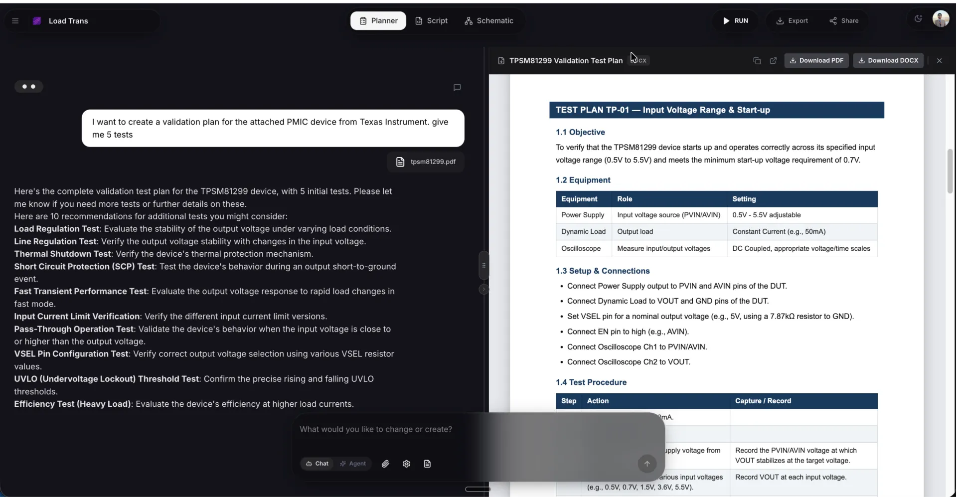
From datasheet to test plan
Upload a chip datasheet and TestFlow generates the full structured test plan, parameters, limits, and instrument requirements included. No more building 1,500-line scripts by hand.
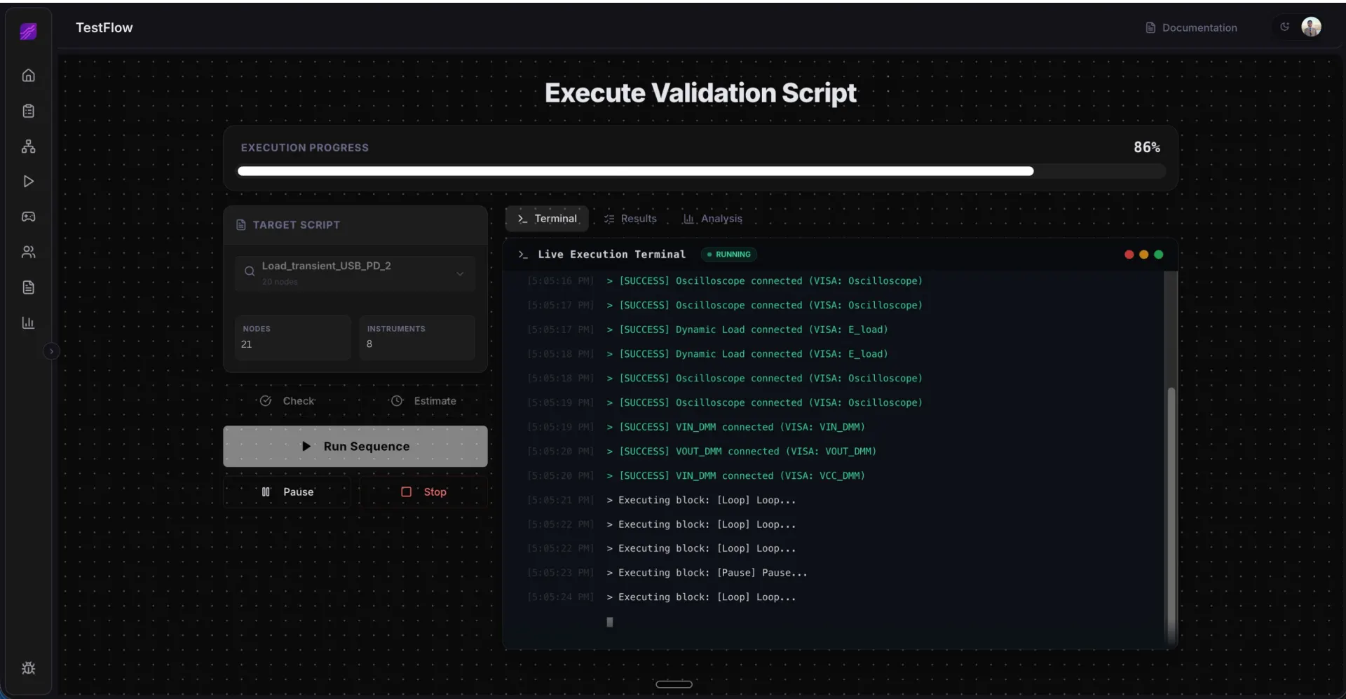
Multi-instrument sequencing
Your Tektronix scope, power supply, signal generator, DMM, and load run together as one sequence. Pass/fail logic, retries, and limits applied to every measurement, not just stored in CSVs.
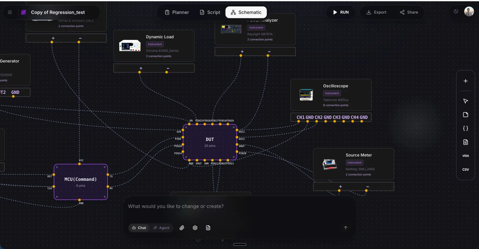
Wire the bench, not the script
Define your bench setup visually. TestFlow handles the SCPI wiring underneath.
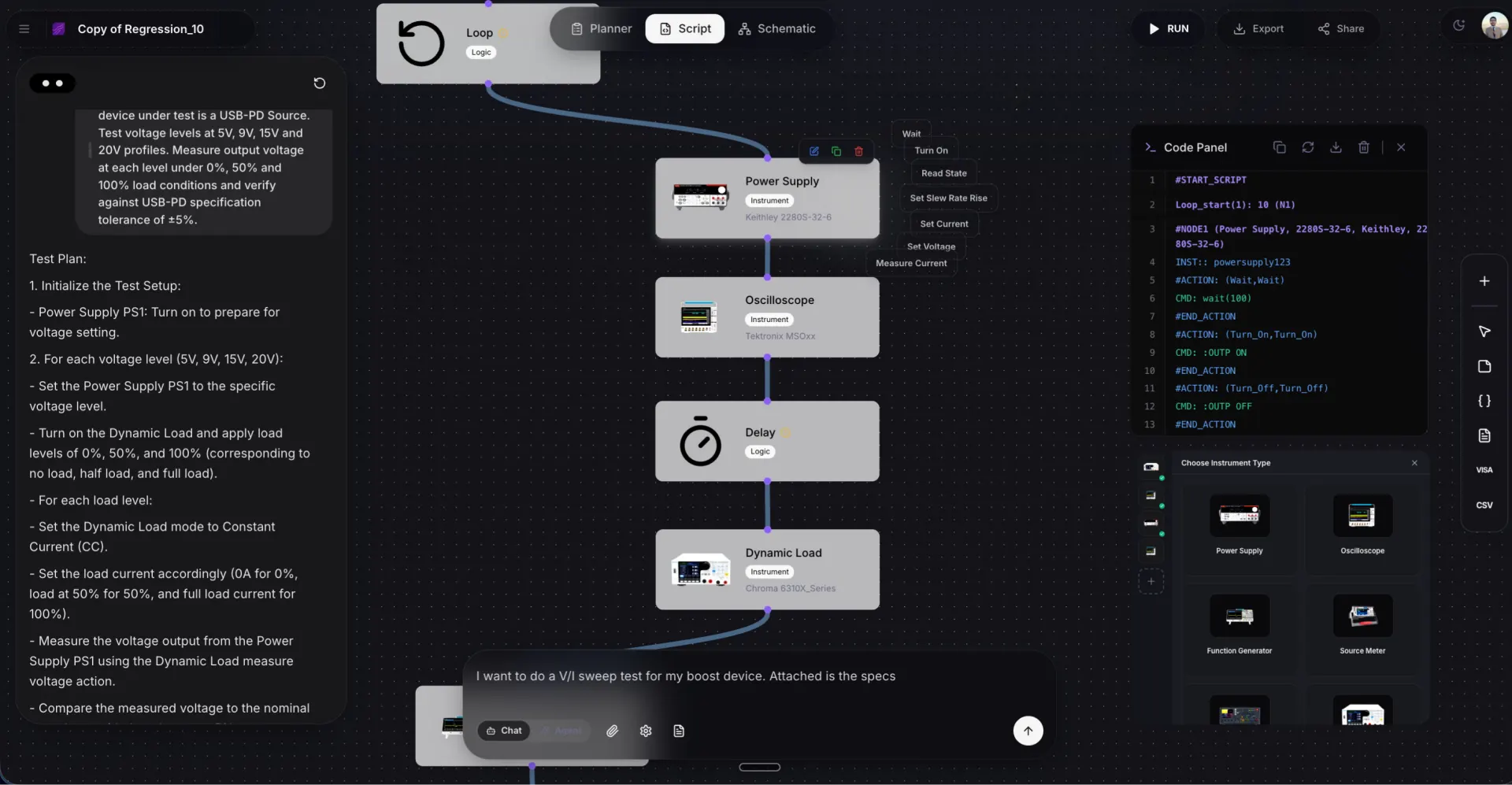
Direct SCPI, without the boilerplate
Interactive instrument control for debugging, the part you used PyVISA for, built in.
Professional reports, generated
Every run produces a structured validation report with charts, pass/fail summaries, and data lineage. No Word, no manual assembly.
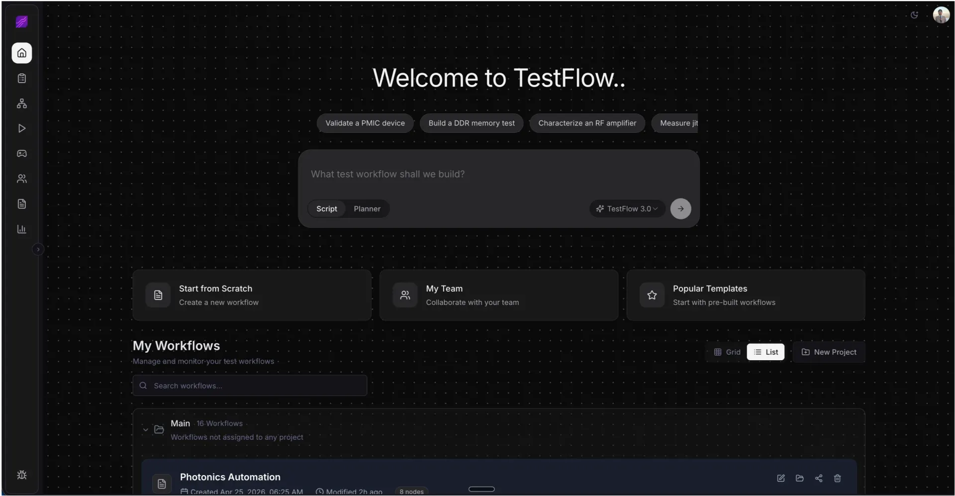
Ready to retire the 1,500-line Python script?
Coordinate your Tektronix scope and the rest of your bench in one structured workflow. See how validation teams use TestFlow.
Summary
Automating a Tektronix oscilloscope with Python is straightforward: install PyVISA, connect via USB or LAN, send SCPI commands for configuration, and query measurements or raw waveform data. The code in this guide covers every common measurement task.
For teams building structured validation workflows across multiple instruments, TestFlow handles the workflow layer, so your engineers spend time validating chips, not maintaining infrastructure.